
(This article was originally published at The DO Loop, and syndicated at StatsBlogs.)
This article describes how to implement the truncated normal distribution in SAS. Although the implementation in this article uses the SAS/IML language, you can also implement the ideas and formulas by using the DATA step and PROC FCMP. For reference, I recommend the Wikipedia article on the truncated normal distribution.
The truncated normal distribution contains two parts: a normal distribution N(μ, σ), and an interval of truncation [a, b]. Denote the four-parameter truncated normal distribution by TN(μ, σ, a, b). There are four essential functions that you need when you are working with a statistical distribution. You need to know how to generate random values, how to compute the density (PDF), how to compute the cumulative distribution (CDF), and how to compute quantiles (inverse CDF).
The example in this article specifies a finite interval, which results in doubly-truncated distribution. However, the functions are written to support a one-sided truncation. To generate a distribution that is truncated on the right, specify a = .M so that the truncation interval is (–∞, b]. To generate a distribution that is truncated on the left, specify b = .P so that the truncation interval is [a, ∞).
Random values of the truncated normal distribution
There are two ways to generate random values. The most intuitive method is an acceptance-rejection algorithm: simulate X ~ N(μ, σ) and then reject and discard any values that are outside the interval [a, b]. That technique works well when the probability that X is in the interval [a, b] is reasonably large, but there are general issues that you have to overcome when you implement an acceptance-rejection algorithm in a vector language.
The inverse CDF method for random number generation is easier to implement. If F is the (cumulative) distribution function, then the following steps generate a random variate for the truncated distribution on [a, b]:
- Generate a uniform random value u in the interval [F(a), F(b)].
- Compute the quantile (inverse CDF) for u. That is, compute x = F–1(u).
proc iml;
/* Random sample from TN on [a,b] by using inverse CDF method */
start randTN(N, mu, sigma, a, b);
   /* Support one-sided truncation. Define Phi(.M)=0 and Phi(.P)=1 */
   cdf_a = choose(a=., 0, cdf("Normal", a, mu, sigma));  /* Phi(a) */
   cdf_b = choose(b=., 1, cdf("Normal", b, mu, sigma));  /* Phi(b) */
   u = j(N,1,.);
   call randgen(u, "Uniform");           /* U ~ U(0,1) */
   z = cdf_a + (cdf_b - cdf_a)*u;        /* Z ~ U(Phi(a), Phi(b)) */
   x = quantile("Normal", z, mu, sigma); /* x always in [a,b] */
   return(x);
finish;

/* test: generate 1,000 random values from the truncated normal */
call randseed(12345);
mu = 1; sigma = 0.8;  a = 0;  b = 3;     /* parameters of the distribution */
x = randTN(1000, mu, sigma, a, b);
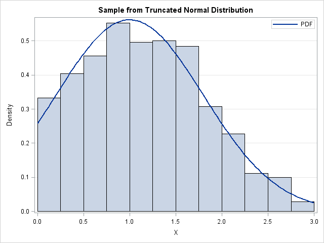
A histogram of the random sample is shown at the top of this post. The histogram is overlaid with a curve that shows the PDF for the truncated normal distribution, which is computed in the next section.
The PDF for the truncated normal distribution
Computing the density function for the truncated normal distribution is easy. You simply use the usual normal PDF on [a, b], but scale the density function so that it integrates to one:
start pdfTN(x, mu, sigma, a, b);
   /* Support one-sided truncation. Define Phi(.M)=0 and Phi(.P)=1 */
   cdf_a = choose(a=., 0, cdf("Normal", a, mu, sigma));  /* Phi(a) */
   cdf_b = choose(b=., 1, cdf("Normal", b, mu, sigma));  /* Phi(b) */
   return( pdf("Normal", x, mu, sigma) / (cdf_b - cdf_a) );
finish;

/* test: generate PDF on [a, b] */
t = do(a, b, (b-a)/100);
y = pdfTN(t, mu, sigma, a, b);
The CDF for the truncated normal distribution
You can express the CDF for the truncated normal distribution in terms of the CDF for the normal distribution. You just need to translate and scale the normal CDF appropriately:
start cdfTN(x, mu, sigma, a, b);
   /* Support one-sided truncation. Define Phi(.M)=0 and Phi(.P)=1 */
   cdf_a = choose(a=., 0, cdf("Normal", a, mu, sigma));  /* Phi(a) */
   cdf_b = choose(b=., 1, cdf("Normal", b, mu, sigma));  /* Phi(b) */
   y = (cdf("Normal", x, mu, sigma) - cdf_a)/ (cdf_b - cdf_a);
   /* If x < a, return 0. If x > b, return 1. */
   if a^=. then do;
      idx = loc(x < a); if ncol(idx)>0 then y[idx] = 0;
   end;
   if b^=. then do;
      idx = loc(x > b); if ncol(idx)>0 then y[idx] = 1;
   end;
   return( y );
finish;

/* test: generate CDF on [a, b] */
t = do(a, b, (b-a)/100);
cdf = cdfTN(t, mu, sigma, a, b);
Quantiles for the truncated normal distribution
Once again, it is easy to compute quantiles of the truncated normal in terms of quantiles of the normal distribution. You just have to scale the normal CDF function appropriately:
start QuantileTN(p, mu, sigma, a, b);
   /* Support one-sided truncation. Define Phi(.M)=0 and Phi(.P)=1 */
   cdf_a = choose(a=., 0, cdf("Normal", a, mu, sigma));  /* Phi(a) */
   cdf_b = choose(b=., 1, cdf("Normal", b, mu, sigma));  /* Phi(b) */
   return( quantile("Normal", cdf_a + (cdf_b - cdf_a)*p, mu, sigma) );
finish;

q = quantileTN(y, mu, sigma, a, b);
Conclusions
The PDF, CDF, QUANTILE, and RAND functions in SAS support distributions that arise often in practice. As shown in this article, you can use these basic distributions as building blocks to define new distributions, such as the truncated normal distribution or the folded normal distribution.
Truncated normal distributions arise in various regression models, such as regression models for the heights of soldiers in the military because there are often height limits for recruits. You can also use the truncated normal distribution to model student scores on standardized tests such as the SAT, for which 200 is the lowest possible score on each test.
Please comment on the article here: The DO Loop
